Laboratory of group mind

This chapter serves as a short and friendly introduction to the formalism used throughout the thesis. As discussed in the introduction, a persistent tension runs through the social sciences: methodological individualists seek to explain social behavior by reducing it to individual preferences, beliefs, or values, while group realists argue that social groups possess irreducible properties that shape outcomes in their own right.

This tension reappears in modeling, though often in subtler ways. Schumpeter's focus on individual decision-making helped lay the groundwork for rational choice theory and game theory §1.1. Meanwhile, social scientists inspired by Simmel's idea of duality used bipartite graphs to represent individuals and their affiliations. While such models acknowledge social context, they often treat groups as metadata on individuals rather than as entities with dynamics of their own. Hence, these models fail to capture the multiscale feedback between individuals and institutions, which could be thought of as a stronger reading of Simmel's duality.

One domain where this modeling tension is especially clear is the problem of cooperation (§1.1.1). If evolution favors selfish individuals---whether rational agents or self-replicating genes---how does large-scale cooperation emerge, especially among unrelated individuals? A common answer is positive assortment: cooperators tend to interact more often with one another than with defectors. This thesis can be read as a modeling ontribution to that broader puzzle.

We close the chapter by introducing the master equation formalism used in Chapter GroupSkills, along with its group-based extension developed in Chapter Coevo.

Abstract

We combine two families of models to explore the complexity of groups and institutions; contagion models and evolutionary game theory models. Both have recently been extended using hypergraph and approximate master equation formalism to represent group dynamics. We first introduce mean-field approaches, how they are used in evolutionary game theory, before moving to (approximate) master equations.

Mean-field theory

Many classical models of population biology, epidemiology, and the social sciences rely on mean-field theory, which assumes that each part of the system interacts only with the average or expected state of the others---thereby ignoring structural and dynamical correlations. In this approximation, local fluctuations and heterogeneity are smoothed out, allowing for simpler, often analytically tractable models. A well-known example is the Lotka-Volterra model, where predator-prey interactions are modeled as random encounters between a predator population, , and a prey population, , with interaction rates proportional to their average population sizes [@lotka_contribution_1909; @volterra_variations_1928; @rosenzweig_graphical_1963]. We can represent these modeling assumptions using compartments, where each compartment tracks the size of a population, and the equations describe the flow of individuals between them (see Fig. 1.1). We might think of as the Canadian Lynx and as Hares in the following

where is the rate of hare reproduction, is the rate at which lynx consume hares, is a conversion factor of how many hares are needed to support one lynx, and is the lynx's (natural) death rate. Inspired by chemistry, one can think of a reaction happening at a rate proportional to the system's average state, similar to how stoichiometry determines reaction proportions. Mean-field theory extends this idea by replacing individual interactions with an average effect---like in the law of mass action, where reaction rates depend on mean concentrations rather than tracking every molecule.

The problem of cooperation

The prisoner's dilemma (PD) epitomizes how cooperation was problematized in the social sciences. In classical games, the story is about a pair of individuals who must choose their next move, weighing their choice with an underlying utility function that specifies their preferences over every action profile. Players are assumed to be consistent in their utility functions and knowledge of their opponent's strategy options. Beyond the story that we will not recite here, PD is about the following (generic) payoff matrix

where . Indeed, say a cooperator, Alice, meets another cooperator; she gets , where c and b are the costs and benefits of the encounter's payoff, generally defined. But if Alice meets a defector, say Bob, she pays a cost, , while Bob gets . If both individuals defect, they both get . If and , we have , which effectively means that mutual cooperation would be better than defection (as long as ). Yet, since each is considering what the other will do, Bob and Alice are incentivized to defect (). Since both players believe the other will defect, and that , the only logical option is mutual defection. In games where both players have no benefit from adopting strategies besides mutual defection, the game is said to have a single Nash equilibrium (there could be many). More precisely, since , this is a strict Nash equilibrium, that is, mutual cooperation performs better than the average of the payoffs when one player defects and the other cooperates.

The Nash equilibrium is a simple mathematical result, but it has often been interpreted as proof that self-interested individuals must be tamed---since no one will unilaterally deviate from mutual defection without external incentives [@smaldino_modeling_2023]. By "tamed", we mean that later models showed how cooperation can emerge when agents face punishment threats, such as state intervention. Although we now know there are many ways out of the Prisoner's Dilemma, this line of reasoning influenced scholars like Garrett Hardin in formulating the tragedy of the commons: the idea that rational individuals will overuse and deplete shared resources, such as fisheries or grazing land [@hardin_tragedy_1968]. One could say that simple models of rationality--by assuming selfishness--helped create their own tragedy: shaping institutions that expect defection, discourage trust, and crowd out local cooperation.

The evolution of cooperation

Whereas classical games frame the problem of cooperation in terms of strategies, rationality, and mind reading, evolutionary game theory examines populations where behavioral strategies are inherited, and individual fitness is determined by how common these strategies are within the population. That is, evolutionary game theory is concerned with situations where the consequence of a variable characteristic depends on its frequency in the population, or frequency dependence. In this thesis, we will be particularly interested in how frequency dependence in structured population importantly define the scope of group interactions. Stated bluntly, group interactions can be thought as the fitness of certain traits, not people, based on the joint influence norms and individual psychology in a group-structured population.

Evolutionary game theory is rooted in genetics, with alleles (or genotypes) co-varying with heritable behavioral programs, or strategies [@hamilton_genetical_1964]. A key simplifying assumption is that single alleles code for behaviors. We will later discuss cultural variants, typically transmitted through social transmission. Social learning can occur in multiple directions---vertically (from parents to offspring), horizontally (among peers), or diagonally (from relatives such as uncles). Humans are unique in that individuals also adopt behaviors by emulating those who are perceived as more successful or prestigious, referred to as success- and prestige-biased transmission. But for now, it is useful to understand where the notion of fitness comes from before applying it to cultural systems. In Chapter 4, we explore the consequences of groups copying the institutions of more successful groups, based on perceived fitness within a contagion context

The replicator dynamics is a key result in evolutionary game theory that will allow us to connect literature from cultural evolution with that of public good games (PGGs) on networks

where is the combined fitness of strategy , which is the product of survival and the average number of zygotes it produces.[^3] The average fitness of the population is denoted as . The replicator dynamics capture a central concept in natural selection; variation is essential, and it is maximized when . As we have seen, traits are inherited across generations, making variation a crucial component of evolutionary change. More generally, for a population with multiple strategies, the change in frequency can be written as (see the Appendix for the full derivation). This equation illustrates that a trait with above-average fitness will increase in frequency, while one with below-average fitness will decline. The magnitude of the ratio reveals that the rate of change in frequency is proportional to how much a trait's fitness deviates from the population's mean fitness.

To illustrate the usefulness of the replication dynamics, consider the following Hawk-Dove (or Snowdrift) game, where at each round a pair of individuals fights over a non-divisible resource. In this case, the Hawk and Dove strategies can be summarized with the following payoff matrix

where are the benefits of the resources and are the costs. When a Hawk meets a Hawk, they fight and incur a cost , but when a Hawk meets a Dove, it gains the full resource . Similarly, Dove meets a Dove, they share the resources, but when a Dove meets a Hawk, it gets nothing. We write the expected payoff for a Hawk as $W(H) = p(V-C)/2 + (1-p)V}, while the expected payoff for a Dove is $W(D)=p(0) + (1-p)V/2}. A central question in evolutionary game theory is whether these strategies can coexist in the long run as evolutionary stable states (ESS). The payoffs are linked to evolutionary fitness, as higher payoffs result in passing down the strategies to subsequent generations. To answer this question for a particular strategy, say Hawk, we solve for all values of for which tends to increase

A well-known result is that , that is, the Hawk population dominates below a certain relative benefit-cost ratio. By the same rationale, we find that Dove dominates when , meaning that Hawk-Dove can coexist as an ESS when . This result is the same as substituting the expected payoffs into the replicator dynamics equation (with a constant mean fitness) and finding the equilibrium points for a difference equation in one dimension.

Positive assortment and complex networks {#sub.assort}

Both classical and evolutionary game theory suggest that randomness tends to favor the greedy. In a sea of hawks, doves are at a disadvantage. But if doves preferentially seek out other doves, they gain a foothold---an effect known as positive assortment. Nowak & May (1992) demonstrated a version of this in grid-based Prisoner's Dilemma (PD) games, showing that cooperator clusters can emerge to promote cooperation [@nowak_evolutionary_1992]. Yet, Hauert and Doebeli (2004) later observed that spatial structure does not always enhance cooperation; in a grid with uniform neighborhoods, a higher cost-to-benefit ratio is required than in an unstructured population [@hauert_spatial_2004]. These results motivated researchers to investigate more realistic forms of social structures, including heterogeneity in social contacts, to understand their impact on cooperation [@santos_scale-free_2005; @ohtsuki_simple_2006].

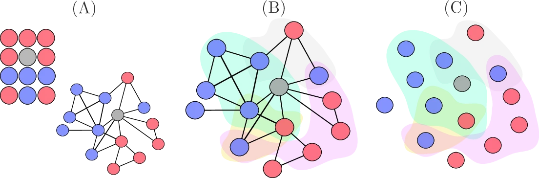
In many real-world social networks, a small number of individuals have disproportionately many connections, while most have relatively few---producing a heavy-tailed degree distribution [@simon_class_1955; @barabasi_emergence_1999]. To capture such heterogeneity, one can group nodes into compartments based on shared attributes (e.g., degree, but also social status, age group, or even evolutionary strategy). Rather than tracking a single, fixed realization of the network, an annealed approximation is often used, wherein links are constantly reshuffled at a rate much faster than the dynamics of interest (e.g., strategy updates or contagion). This constant "reshuffling" of connections means we can effectively work with an ensemble of possible networks that obey certain constraints, thus reflecting these constraints on average, without being locked into any one realization.

Under the annealed approximation, a random contact of a node in compartment leads to a node in compartment with probability

where is the fraction of nodes in compartment , is their average degree, and is the mean degree across all compartments. Because compartments with higher degrees get proportionally more contacts, we capture how diverse connectivity shapes the dynamics, yet maintain a mean-field perspective that avoids simulating a single, static network. By tuning the constraints---e.g., specifying a degree distribution---modelers can systematically isolate and analyze how this structural diversity impacts processes such as cooperation, contagion, or information diffusion.

A well-known mechanism for generating skewed or power-law degree distributions is the preferential attachment growth process [@simon_class_1955; @barabasi_emergence_1999]. In this model, new nodes are more likely to connect to already well-connected nodes, a "rich-get-richer" phenomenon. One common form of the resulting degree distribution is:

where is the number of links that each new node introduces upon joining the network. For large , this distribution converges to a power law:

since for large , we have , and so the demoninator behaves like . In such scale-free networks, the presence of highly connected "hubs" can effectively amplify strategy spreading, bolstering positive assortment among cooperators [@santos_scale-free_2005]. In evolutionary game contexts, these strong correlations among individuals can facilitate the emergence of cooperation. Indeed, there is a threshold condition (where and are benefits and costs, respectively, and is the mean degree) that characterizes when cooperation can invade [@ohtsuki_simple_2006]. Scale-free structure thus makes it easier for cooperative strategies to persist, given that large-degree nodes spread---and reinforce---cooperation more effectively than they would in more homogeneous networks.

Limitations of the mean-field theory

All of the results so far rely on the mean-field assumption, which has its limitations. First, when one population's fequency is too high relative to the other, it can drive the other population to very low levels. However, because the mean-field approach averages over the entire population and assumes smooth, deterministic dynamics, both populations can approach zero asymptotically without ever exactly reaching zero. This occurs provided that the initial conditions and model parameters are such that neither population collapses to zero immediately. The smooth nature of these models does not account for individual-level fluctuations or other factors that could lead to sudden extinction.

Even though individuals interact on complex networks, modeling the dynamics often assumes random mixing, where the interaction network is reshuffled much faster than the unfolding of the dynamics. In this framework, interactions are random, but the units involved can have different characteristics that influence how frequently they interact with each other. Because these interactions are reassigned at each time step, the states of different units become independent over time, "washing out" any correlations between their behaviors. For example, even though Alice, Bob, and Trent might interact more often than others due to their age, they may also form a tightly-knit clique, influencing one another's states in nontrivial ways---an effect that the annealed approximation fails to capture.

To better account for such local dynamical correlations arising from the joint influence of individual node states and higher-order group interactions, we turn to master equations. These equations track the evolution of individual unit states while preserving information about the structure of interactions within the network, offering a more precise description of the system's dynamics than the mean-field approach, which only considers averaged behaviors. In particular, group-centered approximate master equations allow us to describe group-based processes more accurately by shifting focus from individual nodes to classes of groups, distinguished by their size and by the number of cooperators within them.

Modeling with the master equation

With master equations, we are concerned with the probability of the system being in a specific configuration at any given time. That is, rather than asking how the average number of cooperators or defectors changes over time, we care about the full range of possible interactions and how they evolve. For instance, having a configuration with five cooperators and one defector is not necessarily equivalent to its inverse. The exact arrangement matters: a lone defector among cooperators might behave differently than a lone cooperator among defectors. Master equations allow us to keep track of such distinctions. As such, they are exact, in contrast to the group-based master equations we introduce next.

We examine Weidlich and Haag's (1983) Lotka-Volterra master equation model, which extends the prey-predator dynamics to include a refuge habitat where prey are out of reach of predators (Fig. 1.4) [@haag_modelling_2017]. In this model, they show how the refuge habitat contributes to modeling the instability of the Lotka-Volterra cycles against perturbations, resulting in stable cycles instead of unstable closed curves. The modeling of different habitats, and how we can model the effect by taking into within--group composition, as well as the influence of groups interacting with each other, will be a recurrent theme in this thesis.

We represent the system as a time-dependent distribution over states , denoted by . That is, we are concerned with the probability of having in the open-space habitat, prey in the refuge habitat, and predators. As such, master equations are said to describe the time evolution of a system, as we can know the probability of any combination of states at any given time (see Fig. 1.5). We call the occupation number the probability of finding the system in a given state (or, alternatively, the fraction of "systems"), which influence the "probability currents" of transitioning from one occupation state to another adjacent state. One way to visualize such probability currents is as follows

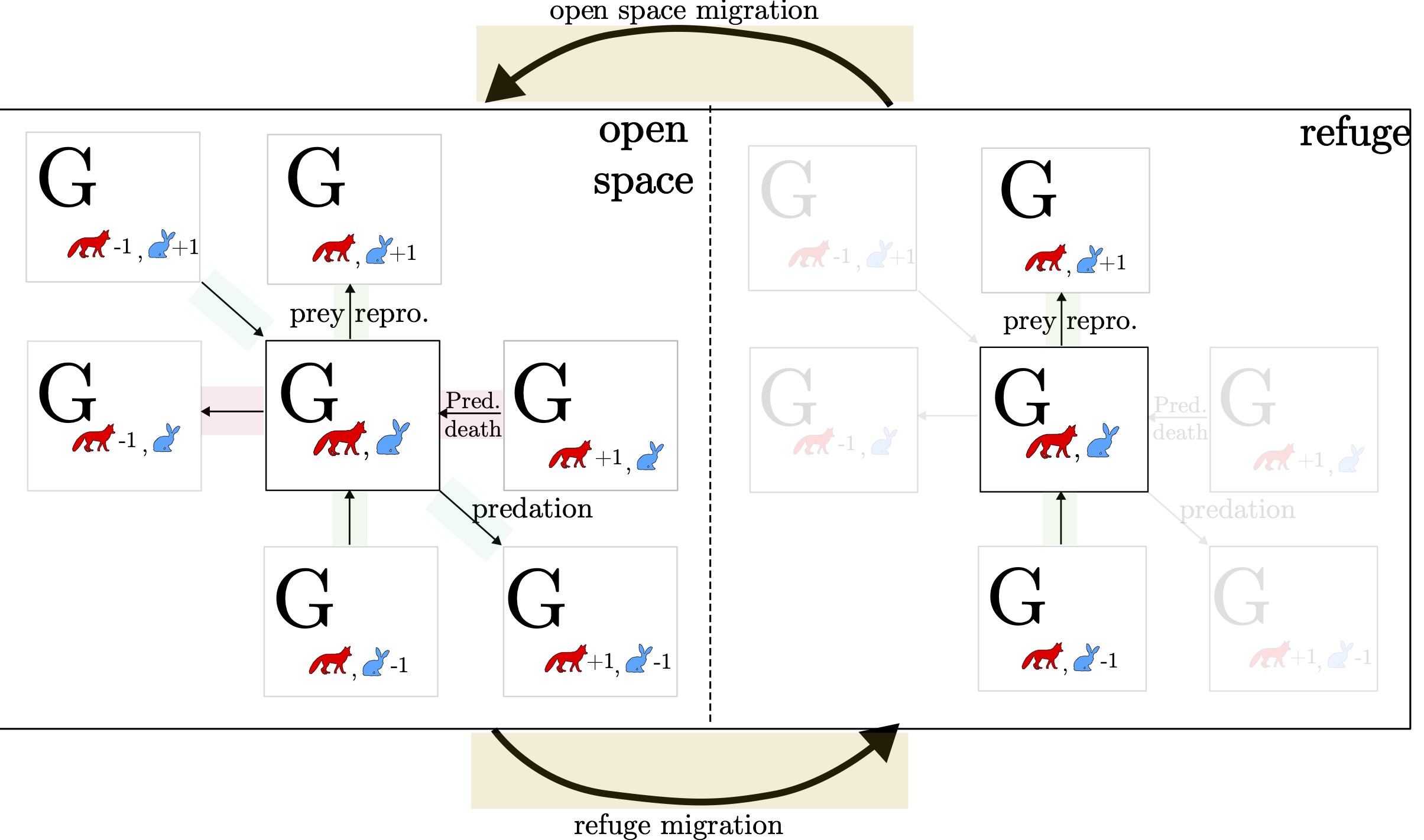
In Fig. 1.4, each compartment represents a state of the entire system. That is, each 'state' corresponds to different configurations, or ensembles, of the (multiverse) system, allowing us to model the probability distribution over all the possible configurations of the system over time. As before, the model retains the same basic information---predation, prey reproduction, and predator deaths---but now we add more details. Specifically, we introduce two distinct habitats in the system. These habitats may influence how the populations interact, which will become important as we model the system's dynamics in more depth. We provide the relevant bits from before but here written as master equations

But master equations are all about balancing our equations so that we have normalization and conservation of our densities. That is, our set of differential equations respects the as well as , respectively. In our equations, it means that what we output with our output probability current (arrows going out) should be balanced with some input currents:

We do the same work for the other parts of the model in the appendix. The important thing is that in the end, we can combine the different parts of the model to get the following master equation:

In figure 1.5, we visualize the systems by either looking at the time dynamics (top rows) or examining the systems at equilibrium (bottom row). The upper left figure demonstrates what is meant by time evolution dynamics, where we can see how the states with 25 predators in the system are becoming increasingly more likely over time. In the upper right figure, we plot the expectation for the different populations, showing

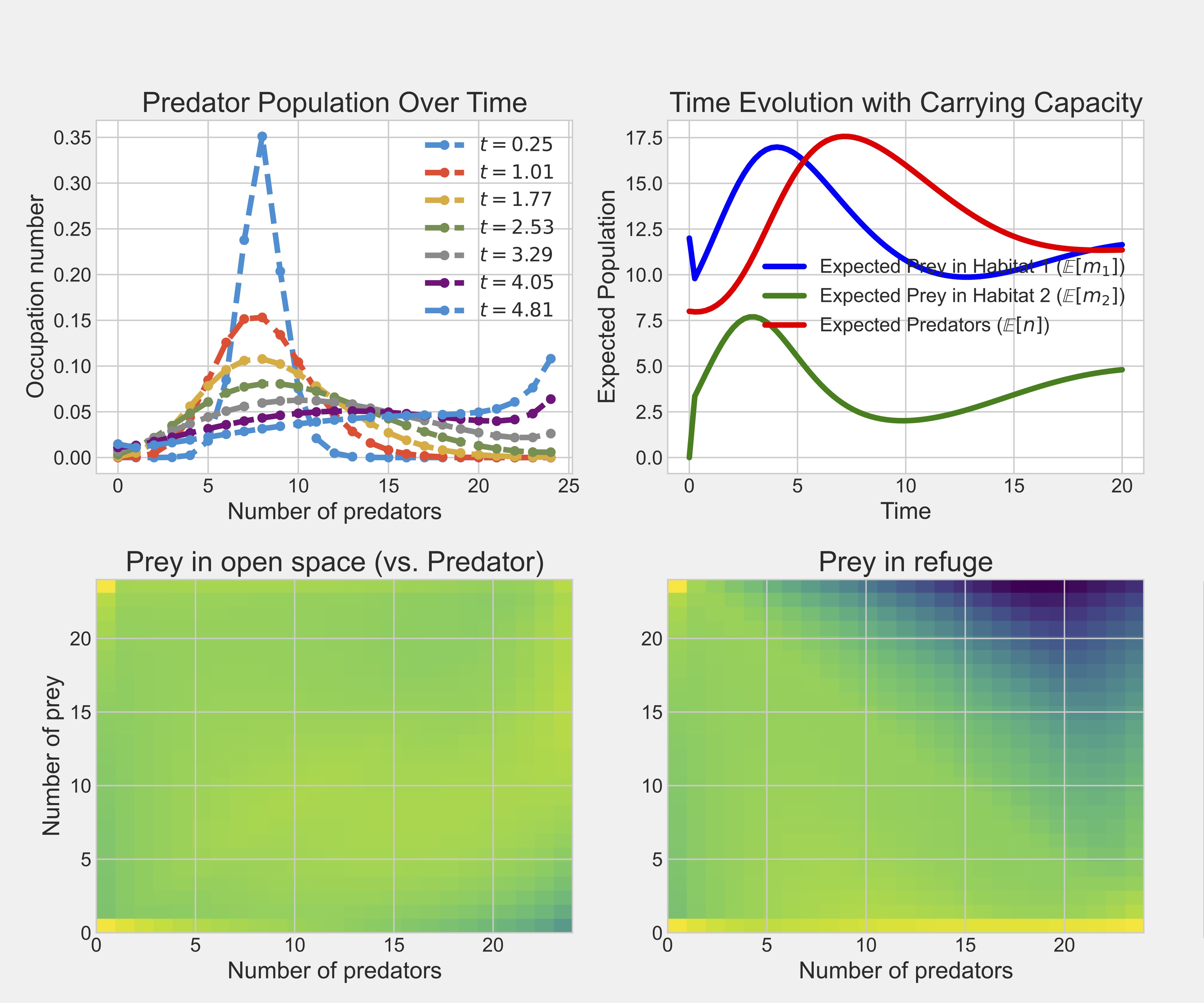
With the probability distributions in hand, we can calculate, for instance, the expected population in the open space habitats by summing over the entire probability distribution (upper right quadrant). But this is a computationally expensive process; for simple binary dynamics, it implies possible states for the systems. For Weidlich and Haag's model, it culminates into possible states, meaning that we need a system with that many coupled ODEs. Alternatively, and more conveniently, we can apply the method of moments to derive an approximate system of ODEs governing the evolution of key statistical moments of the distribution. But our real goal is for the formalism to capture the uniqueness of human group behaviors. To this end, we coarse-grain the dynamics at the mesoscopic level, opening the door to modeling group interactions while preserving crucial details---namely, how individual behavior is shaped by group composition in non-trivial ways. We are willing to trade off the exactness of the master equation in favor of group-based approximations more relevant to social systems.

Group-based master equations

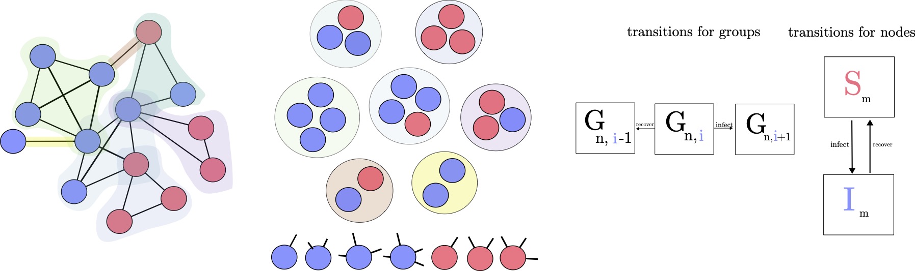
By coarse-graining our set of master equations around relevant subunits, we reduce the system's dimensionality while preserving its core dynamics. We distinguish between equations for individual members---capturing transitions between states within groups--and equations for the groups themselves--tracking how entire group configurations evolve over time. In Fig. 1.6, subunits are shown as circles, which may represent cliques or hyperedges. For instance, we can write 7 member equations to model the internal interactions among group members. These provide a more fine-grained description of the system, whereas group equations summarize how group-level states evolve. We refer to this formalism as group-based master equations (GMEs), in contrast to node-centered master equations where the approximation depends on the states of nodes and their neighbors [@marceau_adaptive_2010].

Building on previous work on approximate master equations [@hebert-dufresne_propagation_2010; @st-onge_master_2021; @st-onge_influential_2022], we extend beyond traditional two-species dynamics (e.g., prey-predator models) to group-based contagion, where individuals transition between Susceptible and Infected states (SIS dynamics). Unlike mean-field models that wash out correlations between individual states, GMEs preserve the exact composition of each group during contagion. This is crucial in settings like airborne virus spread within households or workplaces, where repeated exposure and shared environments lead to strong local reinforcement and non-linear transmission effects.

Coupling between groups arises naturally when individuals belong to multiple groups, creating pathways for contagion or influence to spread indirectly across the system. Originally introduced to model context-dependent contagion [@hebert-dufresne_propagation_2010], this approach has since been applied to settings such as policy co-evolution and collective behavior [@hebert-dufresne_source-sink_2022]. In our framework, such overlap induces dynamic coupling without requiring direct group-to-group interactions--capturing the essence of coupling from our typology in the Interface chapter

We highlight the different places where infection occurs in pink. First, we have the within-group contagion, with the infection rate proportional to the number of susceptible individuals in the group (assuming that groups are of size , so that is the number of susceptible individuals within the group). As before, our master equation must respect the in-flow and out-flow of groups coming into state , based on mechanisms of infection. In the original paper, the infection rate is defined as a non-linear function of the number of infected individuals in the group, or . Second, note that infection also occurs on the first line of equation below, which is an approximation of the fractions of infected nodes of membership m. As such, is treated as a mean field, considering the dynamic correlations between pairs of node-groups (here, nodes in the sense that it refers to the hyperdegree of a node, or the number of groups to which the node belongs). Together, these terms allow us to capture both local (within-group) and global (across-group) mechanisms of infection and recovery, reflecting the multi-scale dynamics typical of real-world group-based contagion.

We have one more place where infection takes place, but this time it happens in the ether (or the mean-field)

On one hand, represents the average infection rate due to the mean-field of groups (i.e. on average, how much of the global population is infected), while represents infections due to expected excess memberships of susceptible nodes (on average, how many infections come from a node having multiple memberships). Although this contributes to the infection, we highlight that this part of the approximation appears in purple (showing up in the last line of the master equation above), where we combine the state transitions of the susceptible nodes in a group due to their membership in other groups, which are modeled via the mean-field quantity . In green, we highlight the transitions corresponding to recovery events, which occur at rate and are proportional to the number of infected individuals .

GMEs provide a more accurate description of spreading processes when contagion depends not only on individual interactions but also on the internal dynamics of groups and how those groups are intertwined. When group sizes are heterogeneous and contagion is superlinear (i.e., $\nu > 1$), the system can exhibit mesoscopic localization: large groups disproportionately drive contagion, lowering the epidemic threshold. This can create hysteresis--where the long-term infection level depends on whether the outbreak began from a small or large seed. In real-world data (e.g., face-to-face contact networks), this implies that early momentum can lock in high infection levels, even if conditions later become unfavorable. Unlike annealed approximations, GMEs assume a quenched group topology--one that remains fixed as dynamics unfold--allowing the model to capture strong within-group correlations and persistent group influence. Groups here may represent contexts where local coordination shapes global dynamics, such as classrooms, teams, or households.

In this thesis, we build on those ideas by combining generalized master equation models with evolutionary game theory, applied to group dynamics. Here, instead of modeling contagion directly, we consider a population of groups playing PGGs, where outcomes depend on trade-offs between individual costs and collective rewards. Importantly, we introduce institutions as explicit actors that collect and redistribute tokens---capturing how institutional policies shape group behavior. One can think of the system as a "multiverse" where all groups play PGGs simultaneously, influencing one another but under differing local conditions set by policy. As in the contagion model, individuals' behaviors are shaped by their group memberships, but now the heterogeneity comes from the variation in institutional rules rather than infection parameters. While we do not explicitly model the rewards players receive, we infer them through their willingness to contribute---cooperation emerges as a function of observed behavior and institutional context. Each group thus acts as a localized game, where players decide whether to cooperate based on what others are doing and how valuable the public good appears to be. In Chapter Interface, we discuss a model in which the incentive to cooperate also depends on the perceived quality of the public good---a crucial feedback often neglected in the existing literature.